R doParallel: How to Parallelize R DataFrame Computations

Parallelizing R dataframe computation is a guaranteed way to shave minutes or even hours from your data processing pipeline compute time. Sure, it adds more complexity to the code, but it can drastically reduce your computing bills, especially if you’re doing everything in the cloud.

R doParallel package provides a significant speed increase to your dataframe calculation while minimizing code changes. It has all you need and more to get your feet wet in the world of dataframe parallelization, and today you’ll learn all about it. After reading, you’ll know what changes you need to make to run your code in parallel, and how your CPU core count affects total compute time and overhead (initialization) time. 

Complete beginner to parallel processing in R? Make sure to read our introduction guide to R doParallel first.

Table of contents:

• How to Get Started with R doParallel
• Baseline - How Slow is Single-Threaded R?
• R doParallel in Action - How to Parallelize DataFrame Aggregations
• R DataFrame Parallelization - Does Compute Time Decrease with More CPU Cores?
• Summing Up R doParallel for DataFrames

How to Get Started with R doParallel

Our introduction guide to parallelism already covered the basic theory and reasons you should care about the topic. Read that piece first if you’re not familiar with the concepts, as this article assumes you have a foundational understanding of R parallelism.

We won’t repeat ourselves here, but to recap:

• R doParallel package enables parallel computing by using the foreach package. This allows you to run foreach loops in parallel, and the computation will be split over multiple CPU cores.
• For R dataframes, this means you’ll have to split them into chunks, where the number of chunks is equal to the number of cores on which your doParallel cluster is running.

If you don’t have these packages installed, make sure to run the following from your R console:

install.packages(c("foreach", "doParallel"))

And that’s it - you’re good to go!

Let’s continue by setting up a baseline - seeing how R performs aggregating on a somewhat large dataset.

Baseline - How Slow is Single-Threaded R?

We’re getting into the good stuff now! The first order of business is to see how R performs on dataset aggregation by default, which will be using dplyr in a single-threaded mode.

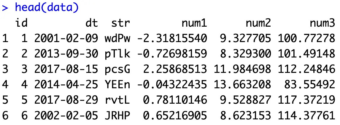
For that, we’ll construct a dataset with 10 million rows. Run this code if you’re following along:

library(dplyr)
library(stringi)
library(cleaner)
library(lubridate)

n <- 10000000

data <- data.frame(
  id = 1:n,
  dt = rdate(n, min = "2000-01-01", max = "2024-01-01"),
  str = stri_rand_strings(n, 4),
  num1 = rnorm(n),
  num2 = rnorm(n, mean = 10, sd = 2),
  num3 = rnorm(n, mean = 100, sd = 10)
)

head(data)

Give it some time, but this is the output you should see:

The core of today’s operation is comparing compute times, so we’ll also declare a helper function time_diff_seconds() that will return a difference in seconds between two datetimes:

time_diff_seconds <- function(t1, t2) {
  return(as.numeric(difftime(t1, t2, units = "secs")))
}

We now have everything needed to find out how slow R is by default.

R dplyr - Single-threaded Execution Benchmark

Many R developers use dplyr, a package that makes data processing a breeze. It’s not the fastest, so we’ll explore one more alternative in the following section.

The goal here is to group the dataset by the str column and calculate averages for all numerical columns. Easy enough, sure, but will take some time due to the amount of rows (10M):

dplyr_bench <- function(dataset) {
  start_time <- Sys.time()
  
  res <- dataset %>%
    group_by(str) %>%
    summarize(
      mean_num1 = mean(num1),
      mean_num2 = mean(num2),
      mean_num3 = mean(num3)
    )
  
  end_time <- Sys.time()
  duration <- time_diff_seconds(end_time, start_time)
  
  print(paste0("Total time:", duration))
  return(res)
}

dplyr_bench_res <- dplyr_bench(data)

This is the output you’ll see after running the above snippet:

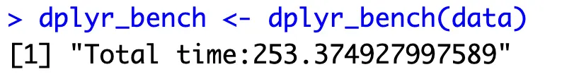
Long story short, it takes a while. Parallelization seems like a good option, but is it the only one? Let’s see what happens if we simply switch the dplyr backend.

R dtplyr - Running dplyr on a Different Backend

The R dtplyr package uses data.table backend, which should aggregate the results faster. The overall runtime will heavily depend on the type of aggregation you’re doing, but on average, you’re almost guaranteed to decrease the compute time.

The best part - the package uses dplyr-like syntax, so the code changes you have to make are minimal. The only important thing to remember is to convert the data.frame to tibble, the rest is pretty self-explanatory:

library(dtplyr)
library(data.table)

dtplyr_bench <- function(dataset) {
  start_time <- Sys.time()
  
  res <- dataset %>%
    lazy_dt() %>%
    group_by(str) %>%
    summarize(
      mean_num1 = mean(num1),
      mean_num2 = mean(num2),
      mean_num3 = mean(num3)
    ) %>%
    as_tibble()
  
  end_time <- Sys.time()
  duration <- time_diff_seconds(end_time, start_time)
  
  print(paste0("Total time:", duration))
  return(res)
}

dtplyr_dataset <- as_tibble(data)
dtplyr_bench_res <- dtplyr_bench(dtplyr_dataset)

Ready for the results? Hold onto your chair just in case:

Yup, you’re reading that correctly. Dtplyr is 20 times faster than dplyr for this simple computation. The difference won’t always be this drastic, but you get the point - there are ways to make R faster without parallelization.

We now have the base results, so let’s see if R doParallel on a data.frame can reduce the compute time even more.

R doParallel in Action - How to Parallelize DataFrame Aggregations

We’ll now dive into the world of R parallel processing, both with dplyr and dtplyr backends. If you’ve read our previous article on R doParallel, you know that R needs a cluster to do its work. A recommended practice is to give it as many cores as you can. Our machine has 12 cores, and we’ll allocate 11 to the cluster.

The dataset then needs to be split into chunks. You’ll have as many chunks as the number of cores you’ve allocated to the cluster.

Then, you can use the foreach() function to apply your data aggregation function to data chunks, all running on separate cores.

Let’s see how this works with dplyr and dtplyr.

R DataFrame Parallelization with dplyr

The dplyr_parallel_bench() function is responsible for setting up the cluster and running the agg_function() function in parallel. We’re also keeping track of the runtime, so we can inspect how much time was taken by computation, and how much by cluster setup.

There’s not much to this function, it’s just a long-ish chunk of easy-to-understand code:

library(doParallel)

dplyr_parallel_bench <- function(dataset) {
  # Function we'll run in parallel
  agg_function <- function(dataset_chunk) {
    dataset_chunk %>%
      group_by(str) %>%
      summarize(
        mean_num1 = mean(num1),
        mean_num2 = mean(num2),
        mean_num3 = mean(num3)
      )
  }
  
  start_time <- Sys.time()
  
  # Cluster setup
  num_cores <- detectCores() - 1
  cl <- makeCluster(num_cores)
  registerDoParallel(cl)
  cluster_time <- Sys.time()
  
  # Split the data into chunks
  chunk_size <- n %/% num_cores
  data_chunks <- split(dataset, ceiling(seq_along(dataset$id) / chunk_size))
  chunk_time <- Sys.time()
  
  # Perform the aggregation in parallel
  parallel_results <- foreach(chunk = data_chunks, .combine = rbind, .packages = "dplyr") %dopar% {
    agg_function(chunk)
  }
  
  # Combine the results from parallel processing
  final_result <- do.call(rbind, parallel_results)
  end_time <- Sys.time()
  
  # Stop the cluster
  stopCluster(cl)
  
  print(paste("Total time:", time_diff_seconds(end_time, start_time)))
  print(paste("Cluster init time:", time_diff_seconds(cluster_time, start_time)))
  print(paste("Chunk time:", time_diff_seconds(chunk_time, cluster_time)))
  print(paste("Processing time:", time_diff_seconds(end_time, chunk_time)))
  
  return(final_result)
}

dplyr_parallel_bench_res <- dplyr_parallel_bench(data)

These are the results we got after running the function:

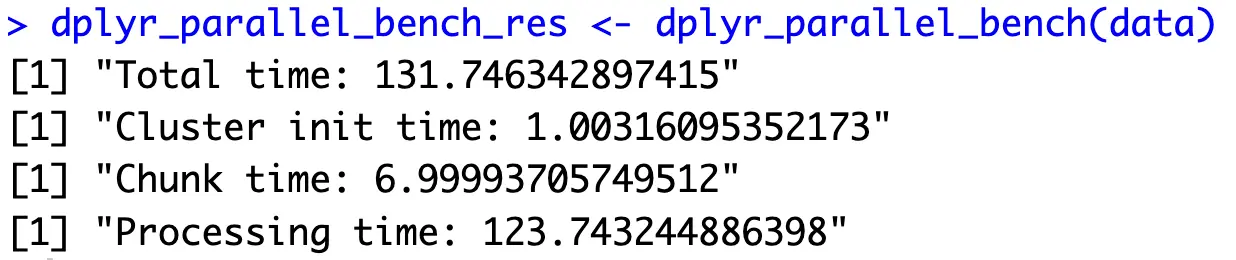
A massive improvement when compared to single-threaded dplyr, but still falls significantly short when compared to the dtplyr implementation.

‍Parallelized dtplyr should then be the fastest, right? Well, let’s see about that.

R DataFrame Parallelization with dtplyr

There aren’t many code changes you need to make. In agg_function(), make sure you call lazy_dt() before doing anything, and also make sure to return the dataset chunk as a tibble.

Then in foreach(), you’ll also want to specify dtplyr as a depending .packages, otherwise some package-specific functions won’t be available.

And that’s it! Here’s the code snippet:

dtplyr_parallel_bench <- function(dataset) {
  # Function we'll run in parallel
  agg_function <- function(dataset_chunk) {
    dataset_chunk %>%
      lazy_dt() %>%
      group_by(str) %>%
      summarize(
        mean_num1 = mean(num1),
        mean_num2 = mean(num2),
        mean_num3 = mean(num3)
      ) %>%
      as_tibble()
  }
  
  start_time <- Sys.time()
  
  # Cluster setup
  num_cores <- detectCores() - 1
  cl <- makeCluster(num_cores)
  registerDoParallel(cl)
  cluster_time <- Sys.time()
  
  # Split the data into chunks
  chunk_size <- n %/% num_cores
  data_chunks <- split(dataset, ceiling(seq_along(dataset$id) / chunk_size))
  chunk_time <- Sys.time()
  
  # Perform the aggregation in parallel
  parallel_results <- foreach(chunk = data_chunks, .combine = rbind, .packages = c("dplyr", "dtplyr")) %dopar% {
    agg_function(chunk)
  }
  
  # Combine the results from parallel processing
  final_result <- do.call(rbind, parallel_results)
  end_time <- Sys.time()
  
  # Stop the cluster
  stopCluster(cl)
  
  print(paste("Total time:", time_diff_seconds(end_time, start_time)))
  print(paste("Cluster init time:", time_diff_seconds(cluster_time, start_time)))
  print(paste("Chunk time:", time_diff_seconds(chunk_time, cluster_time)))
  print(paste("Processing time:", time_diff_seconds(end_time, chunk_time)))
  
  return(final_result)
}

dtplyr_dataset <- as_tibble(data)
dtplyr_parallel_bench_res <- dtplyr_parallel_bench(dtplyr_dataset)

Here are the results we got:

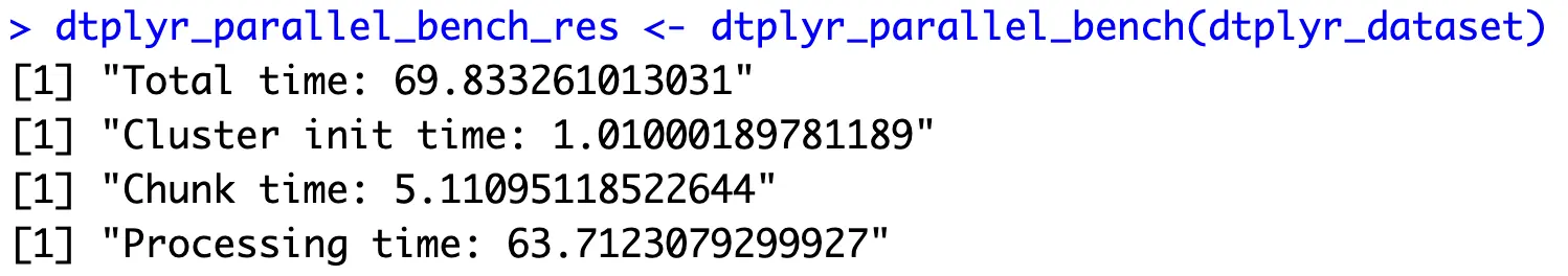
It’s almost twice as fast as parallelized dplyr, but still nowhere near our plain, unparalleled dtplyr implementation. Can we solve this problem by changing the number of cores? Let’s find out.

R DataFrame Parallelization - Does Compute Time Decrease with More CPU Cores?

Any time you’re facing with a slow-running task and want to speed it up via parallelization, it’s important to ask yourself one question - what is the optimal number of CPU cores? R is pretty straightforward as a programming language, so you can easily set up an experiment to find out.

That’s exactly what we’ll do. The core_count_test() function will allow you to configure the maximum number of CPU cores, and will then do our data processing starting at a single core and going up to n_cores_max. The runtime results will be stored in a data.frame, so we can know how much time it took to run the entire thing, and what part of that is due to the overhead (creating a cluster and partitioning the dataset).

Other than that, everything else is R code you’ve seen previously:

core_count_test <- function(dataset, n_cores_max) {
  # Function we'll run in parallel
  agg_function <- function(dataset_chunk) {
    dataset_chunk %>%
      group_by(str) %>%
      summarize(
        mean_num1 = mean(num1),
        mean_num2 = mean(num2),
        mean_num3 = mean(num3)
      )
  }
  
  # Initialize an empty data frame
  time_df <- data.frame(n_cores = c(), total_time = c(), compute_time = c(), overhead_time = c())
  
  # Iterate
  for (n_cores in 1:n_cores_max) {
    start_time <- Sys.time()
    
    # Cluster setup
    cl <- makeCluster(n_cores)
    registerDoParallel(cl)
    cluster_time <- Sys.time()
    
    # Split the data into chunks
    chunk_size <- n %/% n_cores
    data_chunks <- split(dataset, ceiling(seq_along(dataset$id) / chunk_size))
    chunk_time <- Sys.time()
    
    # Perform the aggregation in parallel
    parallel_results <- foreach(chunk = data_chunks, .combine = rbind, .packages = "dplyr") %dopar% {
      agg_function(chunk)
    }
    
    # Combine the results from parallel processing
    final_result <- do.call(rbind, parallel_results)
    end_time <- Sys.time()
    
    # Stop the cluster
    stopCluster(cl)
    
    # Append results
    time_df <- rbind(
      time_df, 
      data.frame(
        n_cores = n_cores, 
        total_time = time_diff_seconds(end_time, start_time), 
        compute_time = time_diff_seconds(end_time, chunk_time), 
        overhead_time = time_diff_seconds(cluster_time, start_time) + time_diff_seconds(chunk_time, cluster_time)
      )
    )
  }
  
  return(time_df)
}

core_count_test_res <- core_count_test(dataset = data, n_cores_max = 12)
core_count_test_res

Running the above snippet will take some time, depending on your hardware configuration. These are the results we got:

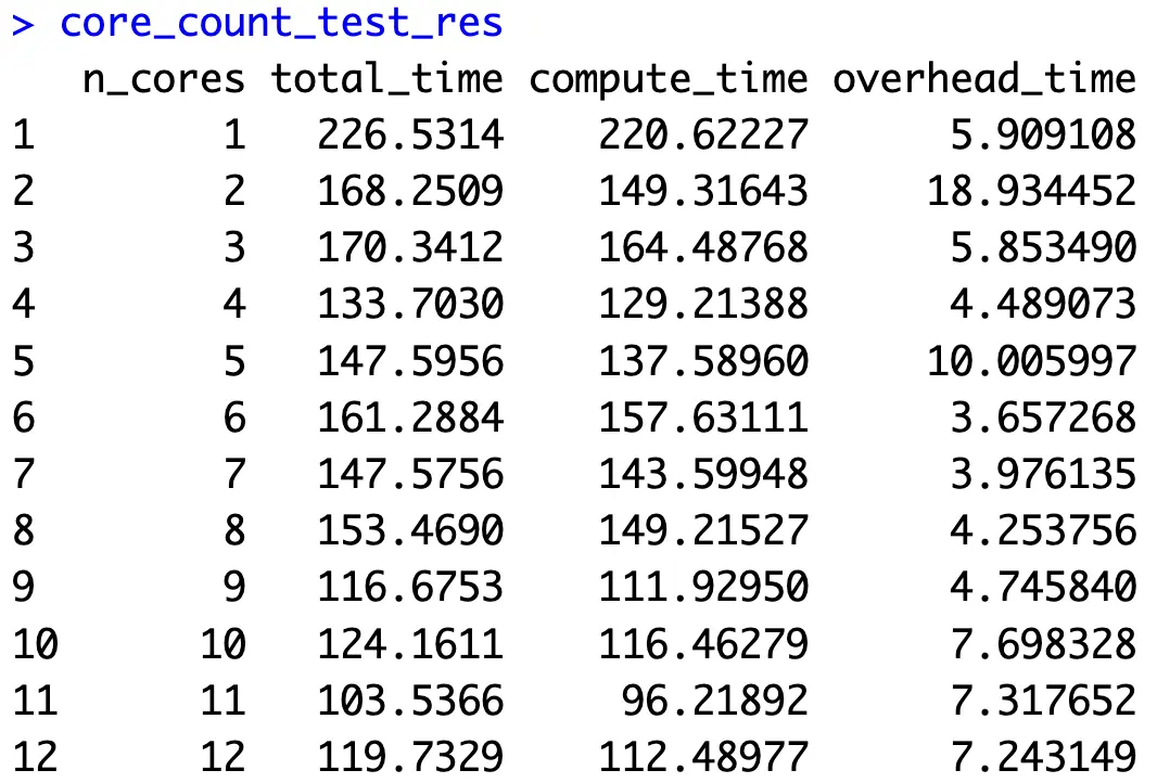
It seems like 11 cores worked best in our case, but let’s inspect the results visually to see if any patterns emerge:

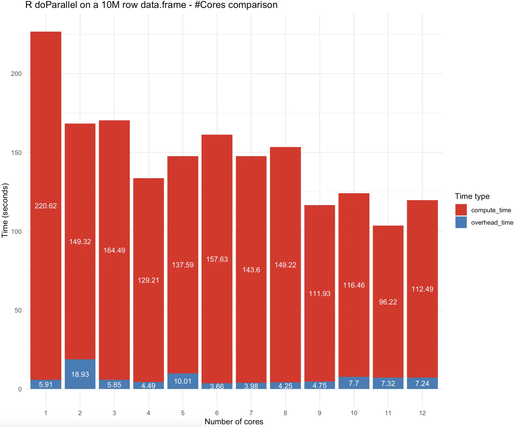
To conclude - 11 CPU cores yielded the results the fastest, but 4-core implementation wasn’t significantly behind. It’s important to note that compute time reduction with increasing number of cores isn’t linear, and sometimes doesn’t make sense at all.

Wondering how we made this stunning stacked bar chart? Here’s a guide to data visualization with R and ggplot2.

Let’s make a brief recap next.

‍

Summing Up R doParallel for DataFrames

In R, parallelization is typically the answer to make your code run faster. That being said, sometimes it isn’t the correct answer since the code is more complex to write. Even if you don’t care about that, a simpler solution might exist that doesn’t require parallelization.

That point was made perfectly clear today. Plain R dtplyr implementation was faster than anything parallelization had to offer. That might not be the case for you though. It’s always important to test all scenarios on your code base, as your data operations might differ in complexity.

We hope you’ve learned something new, and that you’ll all least consider implementing parallel processing for R data frames moving forward.

‍Is your R Shiny application slow? Watch our video on Shiny Infrastructure to find out why.

‍